4 Working with tables
The main library we’ll use is dplyr. We are also using readr for reading files onto R.
library(dplyr)
library(readr)
4.1 Creating and selecting columns
4.1.1 mtcars dataset
Let us begin creating columns or redefining existing ones. For this, we use the mutate() function. It receives a data frame or tibble (mainly via the pipe operator, %>%) and performs a formula for calculating new or existing columns.
We read the data with the read_csv() function from the readr package.
df_mtcars <- read_csv("data/mtcars.csv")##
## ── Column specification ────────────────────────────────────────────────────────
## cols(
## mpg = col_double(),
## cyl = col_double(),
## disp = col_double(),
## hp = col_double(),
## drat = col_double(),
## wt = col_double(),
## qsec = col_double(),
## vs = col_double(),
## am = col_double(),
## gear = col_double(),
## carb = col_double()
## )The data has been obtained from R base and you can read the documentation with ? mtcars.
read_csv() gives us some information about the reading. We can see that all columns belong to class numeric. We can have a more detailed look at the tibble with glimpse(), which shows us the first rows and some info.
df_mtcars %>% glimpse()## Rows: 32
## Columns: 11
## $ mpg <dbl> 21.0, 21.0, 22.8, 21.4, 18.7, 18.1, 14.3, 24.4, 22.8, 19.2, 17.8,…
## $ cyl <dbl> 6, 6, 4, 6, 8, 6, 8, 4, 4, 6, 6, 8, 8, 8, 8, 8, 8, 4, 4, 4, 4, 8,…
## $ disp <dbl> 160.0, 160.0, 108.0, 258.0, 360.0, 225.0, 360.0, 146.7, 140.8, 16…
## $ hp <dbl> 110, 110, 93, 110, 175, 105, 245, 62, 95, 123, 123, 180, 180, 180…
## $ drat <dbl> 3.90, 3.90, 3.85, 3.08, 3.15, 2.76, 3.21, 3.69, 3.92, 3.92, 3.92,…
## $ wt <dbl> 2.620, 2.875, 2.320, 3.215, 3.440, 3.460, 3.570, 3.190, 3.150, 3.…
## $ qsec <dbl> 16.46, 17.02, 18.61, 19.44, 17.02, 20.22, 15.84, 20.00, 22.90, 18…
## $ vs <dbl> 0, 0, 1, 1, 0, 1, 0, 1, 1, 1, 1, 0, 0, 0, 0, 0, 0, 1, 1, 1, 1, 0,…
## $ am <dbl> 1, 1, 1, 0, 0, 0, 0, 0, 0, 0, 0, 0, 0, 0, 0, 0, 0, 1, 1, 1, 0, 0,…
## $ gear <dbl> 4, 4, 4, 3, 3, 3, 3, 4, 4, 4, 4, 3, 3, 3, 3, 3, 3, 4, 4, 4, 3, 3,…
## $ carb <dbl> 4, 4, 1, 1, 2, 1, 4, 2, 2, 4, 4, 3, 3, 3, 4, 4, 4, 1, 2, 1, 1, 2,…Exercise. What are the differences between glimpse(df_mtcars) and df_mtcars %>% glimpse()?
With the first rows we can confirm that all the columns are numerical but we can detect some differences among them. For instance, cyl and the last ones are integer numbers, so they can represent countings, or even categories, since values at vs or am seem only 0 and 1.
We can have more numerical information with summary(), from R base.
summary(df_mtcars)## mpg cyl disp hp
## Min. :10.40 Min. :4.000 Min. : 71.1 Min. : 52.0
## 1st Qu.:15.43 1st Qu.:4.000 1st Qu.:120.8 1st Qu.: 96.5
## Median :19.20 Median :6.000 Median :196.3 Median :123.0
## Mean :20.09 Mean :6.188 Mean :230.7 Mean :146.7
## 3rd Qu.:22.80 3rd Qu.:8.000 3rd Qu.:326.0 3rd Qu.:180.0
## Max. :33.90 Max. :8.000 Max. :472.0 Max. :335.0
## drat wt qsec vs
## Min. :2.760 Min. :1.513 Min. :14.50 Min. :0.0000
## 1st Qu.:3.080 1st Qu.:2.581 1st Qu.:16.89 1st Qu.:0.0000
## Median :3.695 Median :3.325 Median :17.71 Median :0.0000
## Mean :3.597 Mean :3.217 Mean :17.85 Mean :0.4375
## 3rd Qu.:3.920 3rd Qu.:3.610 3rd Qu.:18.90 3rd Qu.:1.0000
## Max. :4.930 Max. :5.424 Max. :22.90 Max. :1.0000
## am gear carb
## Min. :0.0000 Min. :3.000 Min. :1.000
## 1st Qu.:0.0000 1st Qu.:3.000 1st Qu.:2.000
## Median :0.0000 Median :4.000 Median :2.000
## Mean :0.4062 Mean :3.688 Mean :2.812
## 3rd Qu.:1.0000 3rd Qu.:4.000 3rd Qu.:4.000
## Max. :1.0000 Max. :5.000 Max. :8.000For calculating new or existing rows we use mutate(), as mentiobed before. If we only use mutate(), R shows us the data frame with the new calculations on the console, but does not overwrite it. We need to assing the result to the data frame to overwrite the result.
For intance, the weight is given in 1000 lbs. Let’s change the units.
First, we can have a look at the first rows of this column with the function select().
df_mtcars %>%
  select(wt)
## # A tibble: 32 x 1
## wt
## <dbl>
## 1 2.62
## 2 2.88
## 3 2.32
## 4 3.22
## 5 3.44
## 6 3.46
## 7 3.57
## 8 3.19
## 9 3.15
## 10 3.44
## # … with 22 more rowsNow let’s make the calculation.
df_mtcars %>%
  mutate(wt = wt * 1000)
## # A tibble: 32 x 11
## mpg cyl disp hp drat wt qsec vs am gear carb
## <dbl> <dbl> <dbl> <dbl> <dbl> <dbl> <dbl> <dbl> <dbl> <dbl> <dbl>
## 1 21 6 160 110 3.9 2620 16.5 0 1 4 4
## 2 21 6 160 110 3.9 2875 17.0 0 1 4 4
## 3 22.8 4 108 93 3.85 2320 18.6 1 1 4 1
## 4 21.4 6 258 110 3.08 3215 19.4 1 0 3 1
## 5 18.7 8 360 175 3.15 3440 17.0 0 0 3 2
## 6 18.1 6 225 105 2.76 3460 20.2 1 0 3 1
## 7 14.3 8 360 245 3.21 3570 15.8 0 0 3 4
## 8 24.4 4 147. 62 3.69 3190 20 1 0 4 2
## 9 22.8 4 141. 95 3.92 3150 22.9 1 0 4 2
## 10 19.2 6 168. 123 3.92 3440 18.3 1 0 4 4
## # … with 22 more rowsIf there are too many columns is uncomfortable seeing the results. We can use select() and make the pipeline longer.
df_mtcars %>%
  mutate(wt = wt * 1000) %>%
  select(wt)
## # A tibble: 32 x 1
## wt
## <dbl>
## 1 2620
## 2 2875
## 3 2320
## 4 3215
## 5 3440
## 6 3460
## 7 3570
## 8 3190
## 9 3150
## 10 3440
## # … with 22 more rowsThe calculation seems correct. Now, instead of showing the result on the console, we overwrite the result (we don’t use select() now because we want the entire tibble).
df_mtcars <- df_mtcars %>%
  mutate(wt = wt * 1000)
We don’t see anything on the screen but R has changed the column wt. Had we made a mistake and wanted to go back, we would have to execute again the reading of the file or make the opposite calculation.
df_mtcars %>%
  mutate(wt = wt / 1000) %>%
  select(wt)
## # A tibble: 32 x 1
## wt
## <dbl>
## 1 2.62
## 2 2.88
## 3 2.32
## 4 3.22
## 5 3.44
## 6 3.46
## 7 3.57
## 8 3.19
## 9 3.15
## 10 3.44
## # … with 22 more rowsThe documentation explains that vs represents the shape of the engine. It is 0 or 1. Imagine you don’t like this numbers and you want to use 1 and 2. You can easily add 1 to the column.
mtcars %>%
  mutate(vs = vs + 1) %>%
  select(vs)
## vs
## Mazda RX4 1
## Mazda RX4 Wag 1
## Datsun 710 2
## Hornet 4 Drive 2
## Hornet Sportabout 1
## Valiant 2
## Duster 360 1
## Merc 240D 2
## Merc 230 2
## Merc 280 2
## Merc 280C 2
## Merc 450SE 1
## Merc 450SL 1
## Merc 450SLC 1
## Cadillac Fleetwood 1
## Lincoln Continental 1
## Chrysler Imperial 1
## Fiat 128 2
## Honda Civic 2
## Toyota Corolla 2
## Toyota Corona 2
## Dodge Challenger 1
## AMC Javelin 1
## Camaro Z28 1
## Pontiac Firebird 1
## Fiat X1-9 2
## Porsche 914-2 1
## Lotus Europa 2
## Ford Pantera L 1
## Ferrari Dino 1
## Maserati Bora 1
## Volvo 142E 2Remark. Remember to assign the result to the tibble with <- if you want to keep the results. Don’t forget to erase select() in this case.
This change on the column may not seem very useful. It can be more interesting changing the numbers with the real meaning: V-shaped and straight. For this, we need the column to be a character, but it is numeric.
class(df_mtcars$vs)## [1] "numeric"We want to assign these meaning to the numbers and, therefore, the column will be a character, but R will take care of this for us. For changing the values, we use if_else(). We want to say: ‘if vs equals 0, then it will equal “V-shaped”, else “straight”’. We can create and auxiliar column vs_aux for making the change more clear.
df_mtcars %>%
  mutate(vs_aux = if_else(vs == 0, "V-shaped", "straight")) %>%
  select(vs, vs_aux)
## # A tibble: 32 x 2
## vs vs_aux
## <dbl> <chr>
## 1 0 V-shaped
## 2 0 V-shaped
## 3 1 straight
## 4 1 straight
## 5 0 V-shaped
## 6 1 straight
## 7 0 V-shaped
## 8 1 straight
## 9 1 straight
## 10 1 straight
## # … with 22 more rowsRemark. Choose whatever names you want for the columns: it is not necessary to call the auxiliar one vs_aux. And you can overwrite the tibble or not: you are programming, you can always run everything again! =D
The idea of keeping the numbers instead of the character column is that numbers require less space on your computer’s memory. So storing the shape with a numerical code is more efficient. In fact, you have already checked that the column is numerical but it would be better if it were integer.
Exercise. Decide what columns can be stored as integer without losing information and change them. For changing the type of an object or vector you can use as.integer(). For instance:
class(c(4, 6, 1))## [1] "numeric"class(as.integer(4, 6, 1))## [1] "integer"df_mtcars %>%
mutate(
cyl = as.integer(cyl),
vs = as.integer(vs),
am = as.integer(am),
gear = as.integer(gear),
carb = as.integer(carb)
)## # A tibble: 32 x 11
## mpg cyl disp hp drat wt qsec vs am gear carb
## <dbl> <int> <dbl> <dbl> <dbl> <dbl> <dbl> <int> <int> <int> <int>
## 1 21 6 160 110 3.9 2620 16.5 0 1 4 4
## 2 21 6 160 110 3.9 2875 17.0 0 1 4 4
## 3 22.8 4 108 93 3.85 2320 18.6 1 1 4 1
## 4 21.4 6 258 110 3.08 3215 19.4 1 0 3 1
## 5 18.7 8 360 175 3.15 3440 17.0 0 0 3 2
## 6 18.1 6 225 105 2.76 3460 20.2 1 0 3 1
## 7 14.3 8 360 245 3.21 3570 15.8 0 0 3 4
## 8 24.4 4 147. 62 3.69 3190 20 1 0 4 2
## 9 22.8 4 141. 95 3.92 3150 22.9 1 0 4 2
## 10 19.2 6 168. 123 3.92 3440 18.3 1 0 4 4
## # … with 22 more rows4.1.2 Invented dataset
4.1.2.1 Why this is useful
Being able to simulate some random data is useful when you are developing some code but you haven’t receive the final data yet. Nonetheless, because of the project’s timing, you need to keep on working so that you’ll have some code already prepared when you’re data arrives and you don’t need to begin from scratch by then.
4.1.2.2 Simulating data
This branch of Statistics takes several months at University to studying it. But for our purpose we just need some basics concepts.
Imaging you are betting on something and you need a coin. You can use a calculator or R to simulate the results. There is always some function that allows you to get a random number between 0 and 1 (I emphasized random because it requires some time to explain what that means, since nothing is random but controlled by the laws of physics, except maybe the location of an electron). Mathematically, you can use to simulate the results of a coin flip.
runif(10)## [1] 0.958580708 0.175003523 0.465296328 0.431838779 0.524756400 0.001363652
## [7] 0.380046801 0.690146959 0.665239784 0.991097702If you run that on your computer, you’re results will be different (because they are random). Long story short, we can get the same numbers if we fix one thing called seed:
set.seed(1234)
runif(10)
## [1] 0.113703411 0.622299405 0.609274733 0.623379442 0.860915384 0.640310605
## [7] 0.009495756 0.232550506 0.666083758 0.514251141Now you can say that lower than 0.5 results will represent tails and the rest, heads:
set.seed(1234)
results <- runif(10)

library(dplyr)
if_else(results < 0.5, "tails", "heads")
## [1] "tails" "heads" "heads" "heads" "heads" "heads" "tails" "tails" "heads"
## [10] "heads"4.1.2.3 Creating a data frame
You should know that what we have just created is a vector. And vectors can be used as columns on a data frame or tibble. Therefore, we’ll invent some data following this methodology and take advantage of the data for some calculations.
Imagine we have 20 stores, with two dimensions, length and width, the number of customers we receive per day, the daily income and the colors of the walls (between green, red, blue and white (yes, wonderful colors for walls)). Let’s simulate this.
For creating a tibble we use the function tibble(), from the tibble package but available on dplyr. Inside the function we will introduce the vectors with the simulations and the names of the columns. First, the vectors.
number_of_stores <- 20

indices <- 1:number_of_stores # Index: 1, 2, 3, 4, ..., 20

# For the random data we can do the seed thing so that the results will be the same
# for all of us
set.seed(2718)

length_sim <- rnorm(number_of_stores, mean = 7, sd = 1.5)
width_sim <- rnorm(number_of_stores, mean = 10, sd = 2.1)

# For the customers, we assume that the average will be 50.
# You'll learn what a Poisson distribution is later on
customers_daily <- rpois(number_of_stores, lambda = 50)

income_daily <- rnorm(number_of_stores, mean = 2000, sd = 100)

colors <- sample(c("green", "blue", "red", "white"),
                 size = number_of_stores, replace = TRUE)


df_inventado <- tibble(
  ind = indices,
  long = length_sim,
  ancho = width_sim,
  clientes = customers_daily,
  euros = income_daily,
  col = colors
)glimpse(df_inventado)## Rows: 20
## Columns: 6
## $ ind <int> 1, 2, 3, 4, 5, 6, 7, 8, 9, 10, 11, 12, 13, 14, 15, 16, 17, 18…
## $ long <dbl> 7.727768, 5.241214, 8.033535, 6.067075, 5.908894, 6.080340, 8…
## $ ancho <dbl> 12.958071, 10.644176, 10.474705, 7.838526, 11.020973, 9.76414…
## $ clientes <int> 50, 38, 52, 42, 58, 47, 45, 39, 42, 49, 57, 59, 46, 57, 47, 4…
## $ euros <dbl> 2016.820, 1979.281, 1771.956, 2158.435, 1951.960, 1988.361, 2…
## $ col <chr> "white", "blue", "white", "blue", "blue", "green", "green", "…Exercises. Now you make some calculations. You will need mutate(). Remember what has already been explained above. You can decide when to overwrite the data frame with the new calculations or just print them on the console.
Compute the total area of each store.
Calculate how many euros each customer spends, per store.
Calculate how many euros each customer spends on average, in total. Hint. For doing this,
summarise()is very useful and you can read the documentation for learning how to use it. However, you can also use an approach with vectors using$and the functionssum()ormean().If the store is white or blue, reduce its length in 5 meters; else, increase it 10 meters. Hint.
? if_else(). You should also write the condition with%in%. For learning how to do this, play in the console with"white" %in% c("white", "blue")or"red" %in% c("white", "blue")and try to understand what’s happening and how you can use it insidemutate().If all the customers in a day went to the store at the same time, how many squared meters per customer would there be in each store?
Solutions.
# Exercise 1
df_inventado %>%
  mutate(area = ancho * long)

# Exercise 2
df_inventado %>%
  mutate(euros / clientes)

# Exercise 3
df_inventado %>%
  summarise(sum(euros) / sum(clientes))

sum(df_inventado$euros) / sum(df_inventado$clientes)


# Exercise 4
df_inventado %>%
  mutate(nueva_long = if_else(col %in%  c("white", "blue"), long - 5, long + 10)) %>%
  select(nueva_long, long)

# Exercise 5
df_inventado %>%
  mutate(area = long * ancho, sqm_per_cust = area / clientes) %>%
  select(clientes, area, sqm_per_cust)
4.2 Filtering rows
You may know how to apply filters in Excel. In R you can do this too. The goal is to access the rows of a data frame that fulfill certain conditions. We’ll work with an example.
If you have already run library(dplyr), you will be able to use the starwars data frame. You can have a look a it with glimpse() (as you should know by now).
glimpse(starwars)## Rows: 87
## Columns: 14
## $ name <chr> "Luke Skywalker", "C-3PO", "R2-D2", "Darth Vader", "Leia Or…
## $ height <int> 172, 167, 96, 202, 150, 178, 165, 97, 183, 182, 188, 180, 2…
## $ mass <dbl> 77.0, 75.0, 32.0, 136.0, 49.0, 120.0, 75.0, 32.0, 84.0, 77.…
## $ hair_color <chr> "blond", NA, NA, "none", "brown", "brown, grey", "brown", N…
## $ skin_color <chr> "fair", "gold", "white, blue", "white", "light", "light", "…
## $ eye_color <chr> "blue", "yellow", "red", "yellow", "brown", "blue", "blue",…
## $ birth_year <dbl> 19.0, 112.0, 33.0, 41.9, 19.0, 52.0, 47.0, NA, 24.0, 57.0, …
## $ sex <chr> "male", "none", "none", "male", "female", "male", "female",…
## $ gender <chr> "masculine", "masculine", "masculine", "masculine", "femini…
## $ homeworld <chr> "Tatooine", "Tatooine", "Naboo", "Tatooine", "Alderaan", "T…
## $ species <chr> "Human", "Droid", "Droid", "Human", "Human", "Human", "Huma…
## $ films <list> <"The Empire Strikes Back", "Revenge of the Sith", "Return…
## $ vehicles <list> <"Snowspeeder", "Imperial Speeder Bike">, <>, <>, <>, "Imp…
## $ starships <list> <"X-wing", "Imperial shuttle">, <>, <>, "TIE Advanced x1",…Exercise.
- What are the names of the columns?
- What are the classes of each column?
- What are the dimensions of the data frame (number of rows and columns)?
Remark. Remember to use ? starwars to access the documentation.
We can set a condition a take only the rows under this condition. For instance, we want all the character taller than 175cms. You may remember from vector that you can do create a logical vector with this condition doing something like this:
starwars$height > 175## [1] FALSE FALSE FALSE TRUE FALSE TRUE FALSE FALSE TRUE TRUE TRUE TRUE
## [13] TRUE TRUE FALSE FALSE FALSE TRUE FALSE FALSE TRUE TRUE TRUE TRUE
## [25] FALSE TRUE FALSE NA FALSE FALSE TRUE TRUE FALSE TRUE TRUE TRUE
## [37] TRUE FALSE FALSE TRUE FALSE FALSE TRUE TRUE FALSE FALSE FALSE TRUE
## [49] TRUE TRUE FALSE TRUE TRUE TRUE TRUE TRUE TRUE FALSE TRUE TRUE
## [61] FALSE FALSE FALSE TRUE TRUE TRUE FALSE TRUE TRUE TRUE FALSE FALSE
## [73] FALSE TRUE TRUE TRUE TRUE TRUE TRUE TRUE TRUE NA NA NA
## [85] NA NA FALSENow we could see the names of the characters whose associated value in this vector is TRUE. The names of the characters are stored on the first column, name.
starwars$name[starwars$height > 175]## [1] "Darth Vader" "Owen Lars" "Biggs Darklighter"
## [4] "Obi-Wan Kenobi" "Anakin Skywalker" "Wilhuff Tarkin"
## [7] "Chewbacca" "Han Solo" "Jek Tono Porkins"
## [10] "Boba Fett" "IG-88" "Bossk"
## [13] "Lando Calrissian" "Ackbar" NA
## [16] "Qui-Gon Jinn" "Nute Gunray" "Jar Jar Binks"
## [19] "Roos Tarpals" "Rugor Nass" "Ric Olié"
## [22] "Quarsh Panaka" "Bib Fortuna" "Ayla Secura"
## [25] "Mace Windu" "Ki-Adi-Mundi" "Kit Fisto"
## [28] "Adi Gallia" "Saesee Tiin" "Yarael Poof"
## [31] "Plo Koon" "Mas Amedda" "Gregar Typho"
## [34] "Cliegg Lars" "Poggle the Lesser" "Dooku"
## [37] "Bail Prestor Organa" "Jango Fett" "Dexter Jettster"
## [40] "Lama Su" "Taun We" "Wat Tambor"
## [43] "San Hill" "Shaak Ti" "Grievous"
## [46] "Tarfful" "Raymus Antilles" "Sly Moore"
## [49] "Tion Medon" NA NA
## [52] NA NA NAYes, there are some NA things. We’ll talk about than in a few minutes.
Working with vector is efficient but the sintax is verbose. dplyr provide us with a different sintax, data frame - orientated (remember that when doing statistics, data will be mainly stored in tables, therefore we love data frames and working with them <3).
Let’s see how to do this with data frames.
starwars %>%
  filter(height > 175)
## # A tibble: 48 x 14
## name height mass hair_color skin_color eye_color birth_year sex gender
## <chr> <int> <dbl> <chr> <chr> <chr> <dbl> <chr> <chr>
## 1 Darth … 202 136 none white yellow 41.9 male mascu…
## 2 Owen L… 178 120 brown, grey light blue 52 male mascu…
## 3 Biggs … 183 84 black light brown 24 male mascu…
## 4 Obi-Wa… 182 77 auburn, wh… fair blue-gray 57 male mascu…
## 5 Anakin… 188 84 blond fair blue 41.9 male mascu…
## 6 Wilhuf… 180 NA auburn, gr… fair blue 64 male mascu…
## 7 Chewba… 228 112 brown unknown blue 200 male mascu…
## 8 Han So… 180 80 brown fair brown 29 male mascu…
## 9 Jek To… 180 110 brown fair blue NA male mascu…
## 10 Boba F… 183 78.2 black fair brown 31.5 male mascu…
## # … with 38 more rows, and 5 more variables: homeworld <chr>, species <chr>,
## # films <list>, vehicles <list>, starships <list>Doing this we keep all the information about the characters: we have only removed the rows about characters we’re not interested on because of their height.
We can also extend the pipeline and also select only the column of names.
starwars %>%
  filter(height > 175) %>%
  select(name)
## # A tibble: 48 x 1
## name
## <chr>
## 1 Darth Vader
## 2 Owen Lars
## 3 Biggs Darklighter
## 4 Obi-Wan Kenobi
## 5 Anakin Skywalker
## 6 Wilhuff Tarkin
## 7 Chewbacca
## 8 Han Solo
## 9 Jek Tono Porkins
## 10 Boba Fett
## # … with 38 more rowsRemark. Note that we haven’t used the $ notation here. When working with dplyr, R knows where to look for the columns: it knows they are in the data frame. Thus, there is no need to write the name of the data frame followed by $ for accessing columns. Careful with this: it is not a mistake doing it, but works differently and it can lead to errors in some situations. Best practice: don’t do it. Never.
For numerical columns you can use all the comparisons you know: >, >=, <, <=, == and != (for distinct). Notice that you cannot use one single equal sign for comparing. It is very common this mistake but dplyr will properly warn you: just read the messages.
Another example:
starwars %>%
  filter(height != 202) %>%
  nrow()
## [1] 80You can work with character columns:
starwars %>%
  filter(hair_color == "brown")
## # A tibble: 18 x 14
## name height mass hair_color skin_color eye_color birth_year sex gender
## <chr> <int> <dbl> <chr> <chr> <chr> <dbl> <chr> <chr>
## 1 Leia Or… 150 49 brown light brown 19 fema… femin…
## 2 Beru Wh… 165 75 brown light blue 47 fema… femin…
## 3 Chewbac… 228 112 brown unknown blue 200 male mascu…
## 4 Han Solo 180 80 brown fair brown 29 male mascu…
## 5 Wedge A… 170 77 brown fair hazel 21 male mascu…
## 6 Jek Ton… 180 110 brown fair blue NA male mascu…
## 7 Arvel C… NA NA brown fair brown NA male mascu…
## 8 Wicket … 88 20 brown brown brown 8 male mascu…
## 9 Qui-Gon… 193 89 brown fair blue 92 male mascu…
## 10 Ric Olié 183 NA brown fair blue NA <NA> <NA>
## 11 Cordé 157 NA brown light brown NA fema… femin…
## 12 Cliegg … 183 NA brown fair blue 82 male mascu…
## 13 Dormé 165 NA brown light brown NA fema… femin…
## 14 Tarfful 234 136 brown brown blue NA male mascu…
## 15 Raymus … 188 79 brown light brown NA male mascu…
## 16 Rey NA NA brown light hazel NA fema… femin…
## 17 Poe Dam… NA NA brown light brown NA male mascu…
## 18 Padmé A… 165 45 brown light brown 46 fema… femin…
## # … with 5 more variables: homeworld <chr>, species <chr>, films <list>,
## # vehicles <list>, starships <list>And you can combine rules. With commas if you want to have all the rules at the same time: ‘people whose skin color is light and height is greater or equal than 165:’
starwars %>%
  filter(skin_color == "light", height >= 165)
## # A tibble: 7 x 14
## name height mass hair_color skin_color eye_color birth_year sex gender
## <chr> <int> <dbl> <chr> <chr> <chr> <dbl> <chr> <chr>
## 1 Owen La… 178 120 brown, grey light blue 52 male mascu…
## 2 Beru Wh… 165 75 brown light blue 47 fema… femin…
## 3 Biggs D… 183 84 black light brown 24 male mascu…
## 4 Lobot 175 79 none light blue 37 male mascu…
## 5 Dormé 165 NA brown light brown NA fema… femin…
## 6 Raymus … 188 79 brown light brown NA male mascu…
## 7 Padmé A… 165 45 brown light brown 46 fema… femin…
## # … with 5 more variables: homeworld <chr>, species <chr>, films <list>,
## # vehicles <list>, starships <list>If you want say ‘or’ you need to use the | symbol: ‘people whose skin color is light or whose height is lower than 100:’
starwars %>%
  filter(skin_color == "light" | height < 100)
## # A tibble: 18 x 14
## name height mass hair_color skin_color eye_color birth_year sex gender
## <chr> <int> <dbl> <chr> <chr> <chr> <dbl> <chr> <chr>
## 1 R2-D2 96 32 <NA> white, bl… red 33 none mascu…
## 2 Leia Or… 150 49 brown light brown 19 fema… femin…
## 3 Owen La… 178 120 brown, gr… light blue 52 male mascu…
## 4 Beru Wh… 165 75 brown light blue 47 fema… femin…
## 5 R5-D4 97 32 <NA> white, red red NA none mascu…
## 6 Biggs D… 183 84 black light brown 24 male mascu…
## 7 Yoda 66 17 white green brown 896 male mascu…
## 8 Lobot 175 79 none light blue 37 male mascu…
## 9 Wicket … 88 20 brown brown brown 8 male mascu…
## 10 Dud Bolt 94 45 none blue, grey yellow NA male mascu…
## 11 Cordé 157 NA brown light brown NA fema… femin…
## 12 Dormé 165 NA brown light brown NA fema… femin…
## 13 Ratts T… 79 15 none grey, blue unknown NA male mascu…
## 14 R4-P17 96 NA none silver, r… red, blue NA none femin…
## 15 Raymus … 188 79 brown light brown NA male mascu…
## 16 Rey NA NA brown light hazel NA fema… femin…
## 17 Poe Dam… NA NA brown light brown NA male mascu…
## 18 Padmé A… 165 45 brown light brown 46 fema… femin…
## # … with 5 more variables: homeworld <chr>, species <chr>, films <list>,
## # vehicles <list>, starships <list>4.3 Distinct
In Excel you can easily get the different values from a column when selecting it. Imaging that you want all the hair colors available in the Starwars universe, no matter whose hair it is. In this case, you would be interested on the distinct values of the hair_color of the data frame.
There are two ways of doing this: the vectorial way and the dplyr way. Depending on the situation you will need one or the other, so learn both.
4.3.1 R base
Exercise. Get the unique values for the hair_color columns. Remember to use the $ notation for getting the vector and then apply the function unique() to it. You will have a vector with no repeated values.
unique(starwars$hair_color)## [1] "blond" NA "none" "brown"
## [5] "brown, grey" "black" "auburn, white" "auburn, grey"
## [9] "white" "grey" "auburn" "blonde"
## [13] "unknown"Don’t worry too much about that NA thing: we’ll get into that in the next section.
4.3.2 dplyr
As you have seen, applying unique() to a vector you obtain a vector of the different values of the input. But when dealing with exploratory analysis you may want to preserve the tabular format, since it is easy to glance through it as well as export to Excel. For doing this, we use the dplyr function distinct(), which receives a data frame or tibble via the pipe %>% and the name of the columns whose unique values we want to obtain within the brackets.
starwars %>%
  distinct(hair_color)
## # A tibble: 13 x 1
## hair_color
## <chr>
## 1 blond
## 2 <NA>
## 3 none
## 4 brown
## 5 brown, grey
## 6 black
## 7 auburn, white
## 8 auburn, grey
## 9 white
## 10 grey
## 11 auburn
## 12 blonde
## 13 unknownWe can do the same with several columns at the same time:
starwars %>%
  distinct(hair_color, skin_color)
## # A tibble: 50 x 2
## hair_color skin_color
## <chr> <chr>
## 1 blond fair
## 2 <NA> gold
## 3 <NA> white, blue
## 4 none white
## 5 brown light
## 6 brown, grey light
## 7 <NA> white, red
## 8 black light
## 9 auburn, white fair
## 10 auburn, grey fair
## # … with 40 more rowsIn this data frame you have all the different existing combinations between hair_color and skin_color. There is no way of doing this only with unique(), in a vectorial way.
Exercise (also for readr). Get the distinct combinations between eye_color and gender and create a data frame with them. Export this data frame or tibble to a csv file using a function from the readr library. Hint. After running library(readr), write on the console or the script write_ and let the autocompletion propose you some alternatives. Decide which function you should use. Another hint. There are several solutions for exporting the file. Anyway, remember to use ? for reading the help of a function.
new_df <- starwars %>%
  distinct(eye_color, gender)

library(readr)
write_csv(new_df, "new_file_super_cool.csv")
4.4 Some comments about NA
When having a look at the values of hair_color you can see there is something written like NA. This is a symbol used for specifying the generally named missing values and its direct meaning is not available. In several programming languages, like R, this symbol is very important because R works with it in a particular way.
Missing values cannot easily be replace by some other because it will often have meaning. We will mention some examples during the sessions.
Let’s extract the distinct values of that column.
unique_hair_color <- unique(starwars$hair_color)
unique_hair_color
## [1] "blond" NA "none" "brown"
## [5] "brown, grey" "black" "auburn, white" "auburn, grey"
## [9] "white" "grey" "auburn" "blonde"
## [13] "unknown"This NA is the only value not written within ". But the vector is a character vector.
class(unique_hair_color)## [1] "character"If take the first value of the vector, "blonde", it is a character:
class(unique_hair_color[1])## [1] "character"What about the second, which is NA?
class(unique_hair_color[2])## [1] "character"Exercise. Repeat the same procedure with height column and see what class NA belong to this time.
Exercise. Apply the class() function to NA and see the result.
This is very important. NA class is not fixed and can lead you to a lot of problems when reading data.
It is mandatory knowing how to deal with NA values since it can change everything you analyse. For instance, let’s calculate the average height of the characters from Starwars.
mean(starwars$height)## [1] NAThe result of that calculation is NA because when operating with NA the result is always NA, even the most simple thing:
1 + NA## [1] NAYou cannot operate with NA so you need to get rid of it. Some R functions allow you to exclude them adding some commands:
mean(starwars$height, na.rm = TRUE)## [1] 174.358We will now focus on dealing with them in dplyr.
is.na() is a R base function that allows us detecting NA values. Simple example:
vector_with_NA <- c(1, NA, 3)
is.na(vector_with_NA)
## [1] FALSE TRUE FALSEYou can also work denying it, in logical terms:
!is.na(vector_with_NA)## [1] TRUE FALSE TRUEWorking with dplyr is similar:
starwars %>%
  filter(is.na(height))
## # A tibble: 6 x 14
## name height mass hair_color skin_color eye_color birth_year sex gender
## <chr> <int> <dbl> <chr> <chr> <chr> <dbl> <chr> <chr>
## 1 Arvel C… NA NA brown fair brown NA male mascu…
## 2 Finn NA NA black dark dark NA male mascu…
## 3 Rey NA NA brown light hazel NA female femin…
## 4 Poe Dam… NA NA brown light brown NA male mascu…
## 5 BB8 NA NA none none black NA none mascu…
## 6 Captain… NA NA unknown unknown unknown NA <NA> <NA>
## # … with 5 more variables: homeworld <chr>, species <chr>, films <list>,
## # vehicles <list>, starships <list>The contrary:
starwars %>%
  filter(!is.na(height))
## # A tibble: 81 x 14
## name height mass hair_color skin_color eye_color birth_year sex gender
## <chr> <int> <dbl> <chr> <chr> <chr> <dbl> <chr> <chr>
## 1 Luke S… 172 77 blond fair blue 19 male mascu…
## 2 C-3PO 167 75 <NA> gold yellow 112 none mascu…
## 3 R2-D2 96 32 <NA> white, bl… red 33 none mascu…
## 4 Darth … 202 136 none white yellow 41.9 male mascu…
## 5 Leia O… 150 49 brown light brown 19 fema… femin…
## 6 Owen L… 178 120 brown, grey light blue 52 male mascu…
## 7 Beru W… 165 75 brown light blue 47 fema… femin…
## 8 R5-D4 97 32 <NA> white, red red NA none mascu…
## 9 Biggs … 183 84 black light brown 24 male mascu…
## 10 Obi-Wa… 182 77 auburn, wh… fair blue-gray 57 male mascu…
## # … with 71 more rows, and 5 more variables: homeworld <chr>, species <chr>,
## # films <list>, vehicles <list>, starships <list>It is possible to combine rules, as we previously saw.
starwars %>%
  filter(is.na(height) | is.na(hair_color))
## # A tibble: 11 x 14
## name height mass hair_color skin_color eye_color birth_year sex gender
## <chr> <int> <dbl> <chr> <chr> <chr> <dbl> <chr> <chr>
## 1 C-3PO 167 75 <NA> gold yellow 112 none mascu…
## 2 R2-D2 96 32 <NA> white, blue red 33 none mascu…
## 3 R5-D4 97 32 <NA> white, red red NA none mascu…
## 4 Greedo 173 74 <NA> green black 44 male mascu…
## 5 Jabba … 175 1358 <NA> green-tan,… orange 600 herm… mascu…
## 6 Arvel … NA NA brown fair brown NA male mascu…
## 7 Finn NA NA black dark dark NA male mascu…
## 8 Rey NA NA brown light hazel NA fema… femin…
## 9 Poe Da… NA NA brown light brown NA male mascu…
## 10 BB8 NA NA none none black NA none mascu…
## 11 Captai… NA NA unknown unknown unknown NA <NA> <NA>
## # … with 5 more variables: homeworld <chr>, species <chr>, films <list>,
## # vehicles <list>, starships <list>This is useful for making sure that you have all the information you need for an analysis. Suppose you are asked to calculate the BMI (explained during the second session). You need both the height and the mass, so you should check both columns are available.
Exercise. Keep only the rows with both height and mass available and create a new column with the BMI (\(m / h^2\)). Finally select the name of the character and the new column.
starwars %>%
  filter(!is.na(height), !is.na(mass)) %>%
  mutate(mass / (height ^ 2))
## # A tibble: 59 x 15
## name height mass hair_color skin_color eye_color birth_year sex gender
## <chr> <int> <dbl> <chr> <chr> <chr> <dbl> <chr> <chr>
## 1 Luke S… 172 77 blond fair blue 19 male mascu…
## 2 C-3PO 167 75 <NA> gold yellow 112 none mascu…
## 3 R2-D2 96 32 <NA> white, bl… red 33 none mascu…
## 4 Darth … 202 136 none white yellow 41.9 male mascu…
## 5 Leia O… 150 49 brown light brown 19 fema… femin…
## 6 Owen L… 178 120 brown, grey light blue 52 male mascu…
## 7 Beru W… 165 75 brown light blue 47 fema… femin…
## 8 R5-D4 97 32 <NA> white, red red NA none mascu…
## 9 Biggs … 183 84 black light brown 24 male mascu…
## 10 Obi-Wa… 182 77 auburn, wh… fair blue-gray 57 male mascu…
## # … with 49 more rows, and 6 more variables: homeworld <chr>, species <chr>,
## # films <list>, vehicles <list>, starships <list>, mass/(height^2) <dbl>Exercise. Read the help of na.omit() function for removing all the rows with at least one NA value from the starwars data frame. Create a new dataframe with the data. Export the new data frame to a csv file (separated with comma).
4.5 Row numbers
Another way for selecting rows is using a numerical index instead of conditions. Thus, you could access directly the first, third and fifth column of a data frame. This can be done with slice() (also with R base, but we’re not getting into that).
iris %>%
  slice(1:3, 100:103)
## Sepal.Length Sepal.Width Petal.Length Petal.Width Species
## 1 5.1 3.5 1.4 0.2 setosa
## 2 4.9 3.0 1.4 0.2 setosa
## 3 4.7 3.2 1.3 0.2 setosa
## 4 5.7 2.8 4.1 1.3 versicolor
## 5 6.3 3.3 6.0 2.5 virginica
## 6 5.8 2.7 5.1 1.9 virginica
## 7 7.1 3.0 5.9 2.1 virginica4.6 Exercises
Read the file
volpre2019.csvand create a data frame with its data. Name it however you like. It stores data about the volume and the price of lots of products at MercaMadrid.Call the library janitor (install it if needed) and use the
clean_names()function on the data frame (overwrite it).Explore the data frame with the functions you know.
nrow,ncol(you can usedim()instead),glimpse(). Remember to usesummary()too.Count how many
NAvalues there are in thefecha_desdecolumn. Hint. For now it is OK if you just useis.na()for building a logical vector and thensum()for adding the number of cases withNA.Exclude the cases with
fecha_desdeasNAand overwrite the data frame.Get the distinct origins (
desc_origincolumn) of"VACUNO"productos (desc_variedad_2).Select four products from the
desc_variedad_2column and extract the months when they are available (fecha_desde) and the origin. Do it separately for each of them. The final data frame for each product should have two columns. Arrange that data frame bydesc_origin. The function you need isarrange(). Suggestion. For selecting the products, I useddistinct()on the column and thensample_n(4), everything linked with pipes%>%. Read the documentation onsample_n()if needed.
Solutions.
# Exercise 1
library(readr)
df_merca <- read_csv2("data/volpre2019.csv")
## ℹ Using "','" as decimal and "'.'" as grouping mark. Use `read_delim()` for more control.##
## ── Column specification ────────────────────────────────────────────────────────
## cols(
## `Fecha Desde` = col_double(),
## `Fecha Hasta` = col_double(),
## `Cod variedad` = col_character(),
## `Desc variedad` = col_character(),
## `Cod Origen` = col_double(),
## `Desc Origen` = col_character(),
## Kilos = col_double(),
## `Precio frecuente` = col_double(),
## `Precio maximo` = col_double(),
## `Precio minimo` = col_double(),
## `Desc Variedad 2` = col_character()
## )# Exercise 2
library(janitor)##
## Attaching package: 'janitor'## The following objects are masked from 'package:stats':
##
## chisq.test, fisher.testdf_merca <- clean_names(df_merca)
# Exercise 4
sum(is.na(df_merca$fecha_desde))## [1] 5# Exercise 5
df_merca <- df_merca %>%
filter(!is.na(fecha_desde))
# Exercise 6
df_merca %>%
filter(desc_variedad_2 == "VACUNO") %>%
distinct(desc_origen)## # A tibble: 59 x 1
## desc_origen
## <chr>
## 1 BADAJOZ
## 2 BARCELONA
## 3 CACERES
## 4 CUENCA
## 5 LUGO
## 6 MADRID
## 7 NAVARRA
## 8 ORENSE
## 9 PONTEVEDRA
## 10 SALAMANCA
## # … with 49 more rows# Exercise 7
df_merca %>%
distinct(desc_variedad_2) %>%
sample_n(4)## # A tibble: 4 x 1
## desc_variedad_2
## <chr>
## 1 JUREL
## 2 PRECOCINADOS
## 3 BERROS
## 4 POMELOdf_merca %>%
filter(desc_variedad_2 == "CONCHA") %>%
select(fecha_desde, desc_origen) %>%
arrange(desc_origen)## # A tibble: 17 x 2
## fecha_desde desc_origen
## <dbl> <chr>
## 1 20190201 CADIZ
## 2 20190501 CADIZ
## 3 20190601 CADIZ
## 4 20190101 FRANCIA
## 5 20190601 GRAN BRETAÑA
## 6 20190501 GUIPUZCOA
## 7 20190601 GUIPUZCOA
## 8 20190101 HUELVA
## 9 20190501 HUELVA
## 10 20190301 LA CORUÑA
## 11 20190501 LA CORUÑA
## 12 20190101 PONTEVEDRA
## 13 20190201 PONTEVEDRA
## 14 20190301 PONTEVEDRA
## 15 20190401 PONTEVEDRA
## 16 20190501 PONTEVEDRA
## 17 20190601 PONTEVEDRA4.7 Summarizing tables
The main library we’ll use is dplyr.
library(dplyr)We will be working with the storm dataset, stored on the storms.txt file.
library(readr)
df_storms <- read_tsv("data/storms.txt",
                      col_types = cols(
                        name = col_character(),
                        year = col_double(),
                        month = col_double(),
                        day = col_double(),
                        hour = col_double(),
                        status = col_character(),
                        category = col_factor(),
                        wind = col_integer(),
                        pressure = col_integer(),
                        ts_diameter = col_double(),
                        hu_diameter = col_double()
                      ))

glimpse(df_storms)
## Rows: 10,010
## Columns: 11
## $ name <chr> "Amy", "Amy", "Amy", "Amy", "Amy", "Amy", "Amy", "Amy", "A…
## $ year <dbl> 1975, 1975, 1975, 1975, 1975, 1975, 1975, 1975, 1975, 1975…
## $ month <dbl> 6, 6, 6, 6, 6, 6, 6, 6, 6, 6, 6, 6, 6, 6, 6, 6, 7, 7, 7, 7…
## $ day <dbl> 27, 27, 27, 27, 28, 28, 28, 28, 29, 29, 29, 29, 30, 30, 30…
## $ hour <dbl> 0, 6, 12, 18, 0, 6, 12, 18, 0, 6, 12, 18, 0, 6, 12, 18, 0,…
## $ status <chr> "tropical depression", "tropical depression", "tropical de…
## $ category <fct> -1, -1, -1, -1, -1, -1, -1, -1, 0, 0, 0, 0, 0, 0, 0, 0, 0,…
## $ wind <int> 25, 25, 25, 25, 25, 25, 25, 30, 35, 40, 45, 50, 50, 55, 60…
## $ pressure <int> 1013, 1013, 1013, 1013, 1012, 1012, 1011, 1006, 1004, 1002…
## $ ts_diameter <dbl> NA, NA, NA, NA, NA, NA, NA, NA, NA, NA, NA, NA, NA, NA, NA…
## $ hu_diameter <dbl> NA, NA, NA, NA, NA, NA, NA, NA, NA, NA, NA, NA, NA, NA, NA…4.7.1 Exercises
- What can you learn applying
summary()to the tibble? - Which are the different values at the
namecolumn? These are the storms and hurricanes we wil be working with. Create a tibble with one column containing this unique names. - Which are the different available status? Don’t create the tibble: just print it on the console.
- Which are the different combinations between status and pressure?
4.8 Aggregating the data
Exercise 1. How would you calculate the average wind for each status?
## [1] "Tropical depression: 27.2691552062868"## [1] "Tropical storm: 45.8058984910837"## [1] "Hurricane: 85.9689420899385"Taking into account only what has been studied so far about dplyr, we would need to jump into vectors again to calculate the mean for these cases. However we have another function in dplyr for simplifying this: summarise().
df_storms %>%
  filter(status == "tropical depression") %>%
  summarise(avg_wind = mean(wind))
## # A tibble: 1 x 1
## avg_wind
## <dbl>
## 1 27.3df_storms %>%
filter(status == "tropical storm") %>%
summarise(avg_wind = mean(wind))## # A tibble: 1 x 1
## avg_wind
## <dbl>
## 1 45.8df_storms %>%
filter(status == "hurricane") %>%
summarise(avg_wind = mean(wind))## # A tibble: 1 x 1
## avg_wind
## <dbl>
## 1 86.0You can calculate several columns on the fly.
df_storms %>%
  filter(status == "hurricane") %>%
  summarise(avg_wind = mean(wind),
            sd_wind = sd(wind))
## # A tibble: 1 x 2
## avg_wind sd_wind
## <dbl> <dbl>
## 1 86.0 20.3glimpse(df_storms)## Rows: 10,010
## Columns: 11
## $ name <chr> "Amy", "Amy", "Amy", "Amy", "Amy", "Amy", "Amy", "Amy", "A…
## $ year <dbl> 1975, 1975, 1975, 1975, 1975, 1975, 1975, 1975, 1975, 1975…
## $ month <dbl> 6, 6, 6, 6, 6, 6, 6, 6, 6, 6, 6, 6, 6, 6, 6, 6, 7, 7, 7, 7…
## $ day <dbl> 27, 27, 27, 27, 28, 28, 28, 28, 29, 29, 29, 29, 30, 30, 30…
## $ hour <dbl> 0, 6, 12, 18, 0, 6, 12, 18, 0, 6, 12, 18, 0, 6, 12, 18, 0,…
## $ status <chr> "tropical depression", "tropical depression", "tropical de…
## $ category <fct> -1, -1, -1, -1, -1, -1, -1, -1, 0, 0, 0, 0, 0, 0, 0, 0, 0,…
## $ wind <int> 25, 25, 25, 25, 25, 25, 25, 30, 35, 40, 45, 50, 50, 55, 60…
## $ pressure <int> 1013, 1013, 1013, 1013, 1012, 1012, 1011, 1006, 1004, 1002…
## $ ts_diameter <dbl> NA, NA, NA, NA, NA, NA, NA, NA, NA, NA, NA, NA, NA, NA, NA…
## $ hu_diameter <dbl> NA, NA, NA, NA, NA, NA, NA, NA, NA, NA, NA, NA, NA, NA, NA…Exercise 2. For the storms, depressions and hurricanes that took place between 1975 and 1980, create a new column with the mean and standard deviation of the wind. Create a new column substacting the mean from wind and then divide by the standard deviation. Calculate with summarise() the mean and the standard deviation of this new column. What happened?
## # A tibble: 1 x 2
##   `mean(new_column)` `sd(new_column)`
##                <dbl>            <dbl>
## 1          -2.07e-17                1
Exercise 3.
- For the registers where
hu_diameteris notNA, calculate the minimun pressure, the median, the average and the maximum
## # A tibble: 1 x 4
##     min media mediana   max
##   <int> <dbl>   <dbl> <int>
## 1 882 991. 998 1017- Are there more registers below the average or above?
## # A tibble: 1 x 2
##   above_avg below_avg
##       <int>     <int>
## 1      2254      1228
Exercise 4. For the hurricane, calculate the average ts_diameter. Hint. It is not NA.
## # A tibble: 1 x 1
##   media
##   <dbl>
## 1  288.
4.9 A summary
We are now working with an example from the official dplyr documentation, available on the tidyverse site. This notes are just a summary of that page, consisting mainly in copy-pasted paragraphs. The original website may be too technical for our purposes.
The data will used is a dataset containing all 336776 flights that departed from New York City in 2013. The data comes from the US Bureau of Transportation Statistics, it is available in the nycflights13 package and is documented in ? nycflights13.
library(dplyr)
library(nycflights13)

dim(flights)
## [1] 336776 19flights## # A tibble: 336,776 x 19
## year month day dep_time sched_dep_time dep_delay arr_time sched_arr_time
## <int> <int> <int> <int> <int> <dbl> <int> <int>
## 1 2013 1 1 517 515 2 830 819
## 2 2013 1 1 533 529 4 850 830
## 3 2013 1 1 542 540 2 923 850
## 4 2013 1 1 544 545 -1 1004 1022
## 5 2013 1 1 554 600 -6 812 837
## 6 2013 1 1 554 558 -4 740 728
## 7 2013 1 1 555 600 -5 913 854
## 8 2013 1 1 557 600 -3 709 723
## 9 2013 1 1 557 600 -3 838 846
## 10 2013 1 1 558 600 -2 753 745
## # … with 336,766 more rows, and 11 more variables: arr_delay <dbl>,
## # carrier <chr>, flight <int>, tailnum <chr>, origin <chr>, dest <chr>,
## # air_time <dbl>, distance <dbl>, hour <dbl>, minute <dbl>, time_hour <dttm>4.10 Dplyr verbs
Dplyr aims to provide a function for each basic verb of data manipulation:
filter()to select cases based on their values.arrange()to reorder the cases.select()andrename()to select variables based on their names.mutate()andtransmute()to add new variables that are functions of existing variables.summarise()to condense multiple values to a single value.sample_n()andsample_frac()to take random samples.
4.10.1 Filter rows with filter()
filter() allows you to select a subset of rows in a data frame. Firstly, the function receives a tibble (we are doing during the sessions via the %>% command but it is not necessary). Then we also have to write inside the brackets the expression used for rows selection. This expression will be TRUE for the selected rows.
Exercise 1. Select all flights on January 1st.
## # A tibble: 842 x 19
##     year month   day dep_time sched_dep_time dep_delay arr_time sched_arr_time
##    <int> <int> <int>    <int>          <int>     <dbl>    <int>          <int>
##  1  2013     1     1      517            515         2      830            819
##  2  2013     1     1      533            529         4      850            830
##  3  2013     1     1      542            540         2      923            850
##  4  2013     1     1      544            545        -1     1004           1022
##  5  2013     1     1      554            600        -6      812            837
##  6  2013     1     1      554            558        -4      740            728
##  7  2013     1     1      555            600        -5      913            854
##  8  2013     1     1      557            600        -3      709            723
##  9  2013     1     1      557            600        -3      838            846
## 10  2013     1     1      558            600        -2      753            745
## # … with 832 more rows, and 11 more variables: arr_delay <dbl>, carrier <chr>,
## #   flight <int>, tailnum <chr>, origin <chr>, dest <chr>, air_time <dbl>,
## #   distance <dbl>, hour <dbl>, minute <dbl>, time_hour <dttm>
Exercise 2. How many flights departed from JFK airport?
## [1] 111279Exercise 3. How many delayed flights were there?
## [1] 133004Exercise 4. Select the flights with no NA data on the dep_delay column.
## # A tibble: 328,521 x 19
##     year month   day dep_time sched_dep_time dep_delay arr_time sched_arr_time
##    <int> <int> <int>    <int>          <int>     <dbl>    <int>          <int>
##  1  2013     1     1      517            515         2      830            819
##  2  2013     1     1      533            529         4      850            830
##  3  2013     1     1      542            540         2      923            850
##  4  2013     1     1      544            545        -1     1004           1022
##  5  2013     1     1      554            600        -6      812            837
##  6  2013     1     1      554            558        -4      740            728
##  7  2013     1     1      555            600        -5      913            854
##  8  2013     1     1      557            600        -3      709            723
##  9  2013     1     1      557            600        -3      838            846
## 10  2013     1     1      558            600        -2      753            745
## # … with 328,511 more rows, and 11 more variables: arr_delay <dbl>,
## #   carrier <chr>, flight <int>, tailnum <chr>, origin <chr>, dest <chr>,
## #   air_time <dbl>, distance <dbl>, hour <dbl>, minute <dbl>, time_hour <dttm>
4.10.2 Arrange rows with arrange()
arrange() reorders the rows. It takes a data frame, and a set of column names to order by. If you provide more than one column name, each additional column will be used to break ties in the values of preceding columns.
flights %>% arrange(year, month, day)## # A tibble: 336,776 x 19
## year month day dep_time sched_dep_time dep_delay arr_time sched_arr_time
## <int> <int> <int> <int> <int> <dbl> <int> <int>
## 1 2013 1 1 517 515 2 830 819
## 2 2013 1 1 533 529 4 850 830
## 3 2013 1 1 542 540 2 923 850
## 4 2013 1 1 544 545 -1 1004 1022
## 5 2013 1 1 554 600 -6 812 837
## 6 2013 1 1 554 558 -4 740 728
## 7 2013 1 1 555 600 -5 913 854
## 8 2013 1 1 557 600 -3 709 723
## 9 2013 1 1 557 600 -3 838 846
## 10 2013 1 1 558 600 -2 753 745
## # … with 336,766 more rows, and 11 more variables: arr_delay <dbl>,
## # carrier <chr>, flight <int>, tailnum <chr>, origin <chr>, dest <chr>,
## # air_time <dbl>, distance <dbl>, hour <dbl>, minute <dbl>, time_hour <dttm>flights %>% arrange(desc(arr_delay))## # A tibble: 336,776 x 19
## year month day dep_time sched_dep_time dep_delay arr_time sched_arr_time
## <int> <int> <int> <int> <int> <dbl> <int> <int>
## 1 2013 1 9 641 900 1301 1242 1530
## 2 2013 6 15 1432 1935 1137 1607 2120
## 3 2013 1 10 1121 1635 1126 1239 1810
## 4 2013 9 20 1139 1845 1014 1457 2210
## 5 2013 7 22 845 1600 1005 1044 1815
## 6 2013 4 10 1100 1900 960 1342 2211
## 7 2013 3 17 2321 810 911 135 1020
## 8 2013 7 22 2257 759 898 121 1026
## 9 2013 12 5 756 1700 896 1058 2020
## 10 2013 5 3 1133 2055 878 1250 2215
## # … with 336,766 more rows, and 11 more variables: arr_delay <dbl>,
## # carrier <chr>, flight <int>, tailnum <chr>, origin <chr>, dest <chr>,
## # air_time <dbl>, distance <dbl>, hour <dbl>, minute <dbl>, time_hour <dttm>4.10.3 Select columns with select()
Often you work with large datasets with many columns but only a few are actually of interest to you. select() allows you to rapidly zoom in on a useful subset, even using operations.
flights %>% select(year, month, day)## # A tibble: 336,776 x 3
## year month day
## <int> <int> <int>
## 1 2013 1 1
## 2 2013 1 1
## 3 2013 1 1
## 4 2013 1 1
## 5 2013 1 1
## 6 2013 1 1
## 7 2013 1 1
## 8 2013 1 1
## 9 2013 1 1
## 10 2013 1 1
## # … with 336,766 more rowsflights %>% select(year:day) # Everything between year and day## # A tibble: 336,776 x 3
## year month day
## <int> <int> <int>
## 1 2013 1 1
## 2 2013 1 1
## 3 2013 1 1
## 4 2013 1 1
## 5 2013 1 1
## 6 2013 1 1
## 7 2013 1 1
## 8 2013 1 1
## 9 2013 1 1
## 10 2013 1 1
## # … with 336,766 more rowsflights %>% select(-(year:day)) # Everything except year, day and what is in the middle## # A tibble: 336,776 x 16
## dep_time sched_dep_time dep_delay arr_time sched_arr_time arr_delay carrier
## <int> <int> <dbl> <int> <int> <dbl> <chr>
## 1 517 515 2 830 819 11 UA
## 2 533 529 4 850 830 20 UA
## 3 542 540 2 923 850 33 AA
## 4 544 545 -1 1004 1022 -18 B6
## 5 554 600 -6 812 837 -25 DL
## 6 554 558 -4 740 728 12 UA
## 7 555 600 -5 913 854 19 B6
## 8 557 600 -3 709 723 -14 EV
## 9 557 600 -3 838 846 -8 B6
## 10 558 600 -2 753 745 8 AA
## # … with 336,766 more rows, and 9 more variables: flight <int>, tailnum <chr>,
## # origin <chr>, dest <chr>, air_time <dbl>, distance <dbl>, hour <dbl>,
## # minute <dbl>, time_hour <dttm>There are a number of helper functions you can use within select(), like starts_with(), ends_with() and contains(). These let you quickly match larger blocks of variables that meet some criterion. See ?select for more details.
iris %>%
  select(starts_with("Petal")) %>%
  head(6)  # Used for limiting the number of printed rows
## Petal.Length Petal.Width
## 1 1.4 0.2
## 2 1.4 0.2
## 3 1.3 0.2
## 4 1.5 0.2
## 5 1.4 0.2
## 6 1.7 0.4Exercise 5. From flights tibble, select all the columns related to delays (containing something about delays in the name).
## # A tibble: 336,776 x 2
##    dep_delay arr_delay
##        <dbl>     <dbl>
##  1         2        11
##  2         4        20
##  3         2        33
##  4        -1       -18
##  5        -6       -25
##  6        -4        12
##  7        -5        19
##  8        -3       -14
##  9        -3        -8
## 10        -2         8
## # … with 336,766 more rows
You can rename columns while selecting:
flights %>% select(tail_num = tailnum)## # A tibble: 336,776 x 1
## tail_num
## <chr>
## 1 N14228
## 2 N24211
## 3 N619AA
## 4 N804JB
## 5 N668DN
## 6 N39463
## 7 N516JB
## 8 N829AS
## 9 N593JB
## 10 N3ALAA
## # … with 336,766 more rowsBut this is not useful when you want to keep all the variables. For just renaming we use rename().
flights %>% names()## [1] "year" "month" "day" "dep_time"
## [5] "sched_dep_time" "dep_delay" "arr_time" "sched_arr_time"
## [9] "arr_delay" "carrier" "flight" "tailnum"
## [13] "origin" "dest" "air_time" "distance"
## [17] "hour" "minute" "time_hour"flights %>%
rename(tail_num = tailnum) %>%
names()## [1] "year" "month" "day" "dep_time"
## [5] "sched_dep_time" "dep_delay" "arr_time" "sched_arr_time"
## [9] "arr_delay" "carrier" "flight" "tail_num"
## [13] "origin" "dest" "air_time" "distance"
## [17] "hour" "minute" "time_hour"4.10.4 Add new columns with mutate()
The job of mutate() is redefining existing columns or adding new ones.
Exercise 6.
- Define a new column called gain, consisting on substracting
dep_delaytoarr_delay. - Define another one as the average speed (
distancedivided byair_time). Multiply it by 60 to have the result in minutes.
## # A tibble: 336,776 x 21
##     year month   day dep_time sched_dep_time dep_delay arr_time sched_arr_time
##    <int> <int> <int>    <int>          <int>     <dbl>    <int>          <int>
##  1  2013     1     1      517            515         2      830            819
##  2  2013     1     1      533            529         4      850            830
##  3  2013     1     1      542            540         2      923            850
##  4  2013     1     1      544            545        -1     1004           1022
##  5  2013     1     1      554            600        -6      812            837
##  6  2013     1     1      554            558        -4      740            728
##  7  2013     1     1      555            600        -5      913            854
##  8  2013     1     1      557            600        -3      709            723
##  9  2013     1     1      557            600        -3      838            846
## 10  2013     1     1      558            600        -2      753            745
## # … with 336,766 more rows, and 13 more variables: arr_delay <dbl>,
## #   carrier <chr>, flight <int>, tailnum <chr>, origin <chr>, dest <chr>,
## #   air_time <dbl>, distance <dbl>, hour <dbl>, minute <dbl>, time_hour <dttm>,
## #   gain <dbl>, speed <dbl>
mutate() allows you to refer to columns that you’ve just created:
flights %>%
  mutate(
    gain = arr_delay - dep_delay,
    gain_per_hour = gain / (air_time / 60)
)
## # A tibble: 336,776 x 21
## year month day dep_time sched_dep_time dep_delay arr_time sched_arr_time
## <int> <int> <int> <int> <int> <dbl> <int> <int>
## 1 2013 1 1 517 515 2 830 819
## 2 2013 1 1 533 529 4 850 830
## 3 2013 1 1 542 540 2 923 850
## 4 2013 1 1 544 545 -1 1004 1022
## 5 2013 1 1 554 600 -6 812 837
## 6 2013 1 1 554 558 -4 740 728
## 7 2013 1 1 555 600 -5 913 854
## 8 2013 1 1 557 600 -3 709 723
## 9 2013 1 1 557 600 -3 838 846
## 10 2013 1 1 558 600 -2 753 745
## # … with 336,766 more rows, and 13 more variables: arr_delay <dbl>,
## # carrier <chr>, flight <int>, tailnum <chr>, origin <chr>, dest <chr>,
## # air_time <dbl>, distance <dbl>, hour <dbl>, minute <dbl>, time_hour <dttm>,
## # gain <dbl>, gain_per_hour <dbl>4.10.5 Summarise values with summarise()
The last verb is summarise(). It collapses a data frame to a single row.
Exercise 7. Calculate the mean of the delay in the departure. Mind the NAs.
## # A tibble: 1 x 1
##   delay
##   <dbl>
## 1  12.6
This is very powerful when combined with group_by(), not seen yet.
4.10.6 Randomly sample rows with sample_n() and sample_frac()
You can use sample_n() and sample_frac() to take a random sample of rows: use sample_n() for a fixed number and sample_frac() for a fixed fraction.
flights %>% sample_n(10)## # A tibble: 10 x 19
## year month day dep_time sched_dep_time dep_delay arr_time sched_arr_time
## <int> <int> <int> <int> <int> <dbl> <int> <int>
## 1 2013 11 21 616 610 6 918 915
## 2 2013 11 26 1942 1830 72 2134 2046
## 3 2013 5 25 951 959 -8 1142 1203
## 4 2013 10 15 1600 1559 1 1859 1943
## 5 2013 2 27 554 600 -6 835 837
## 6 2013 9 26 1709 1710 -1 1827 1835
## 7 2013 9 17 835 840 -5 950 1022
## 8 2013 3 16 2056 2040 16 2356 2344
## 9 2013 11 10 755 746 9 1052 1050
## 10 2013 10 14 1049 1059 -10 1236 1254
## # … with 11 more variables: arr_delay <dbl>, carrier <chr>, flight <int>,
## # tailnum <chr>, origin <chr>, dest <chr>, air_time <dbl>, distance <dbl>,
## # hour <dbl>, minute <dbl>, time_hour <dttm>flights %>% sample_frac(0.01)## # A tibble: 3,368 x 19
## year month day dep_time sched_dep_time dep_delay arr_time sched_arr_time
## <int> <int> <int> <int> <int> <dbl> <int> <int>
## 1 2013 1 5 950 904 46 1318 1210
## 2 2013 5 30 1741 1732 9 2148 2114
## 3 2013 1 22 1458 1459 -1 1723 1656
## 4 2013 10 4 1245 1249 -4 1459 1512
## 5 2013 2 15 603 600 3 913 906
## 6 2013 2 13 800 810 -10 1009 1007
## 7 2013 7 10 759 800 -1 1008 1021
## 8 2013 10 7 1822 1715 67 2021 1937
## 9 2013 3 28 724 730 -6 1028 1100
## 10 2013 2 13 843 840 3 1154 1143
## # … with 3,358 more rows, and 11 more variables: arr_delay <dbl>,
## # carrier <chr>, flight <int>, tailnum <chr>, origin <chr>, dest <chr>,
## # air_time <dbl>, distance <dbl>, hour <dbl>, minute <dbl>, time_hour <dttm>4.10.7 Commonalities
Notice that all the functions return data frames. Therefore, you can link them all with %>%.
flights %>%
  select(arr_delay, dep_delay) %>%
  filter(arr_delay > 30 | dep_delay > 30) %>%
  summarise(
    arr = mean(arr_delay, na.rm = TRUE),
    dep = mean(dep_delay, na.rm = TRUE)
  )
## # A tibble: 1 x 2
## arr dep
## <dbl> <dbl>
## 1 76.3 72.14.11 Grouped operations
The dplyr verbs are useful on their own, but they become even more powerful when you apply them to groups of observations within a dataset. In dplyr, you do this with the group_by() function. It breaks down a dataset into specified groups of rows. When you then apply the verbs above on the resulting object they’ll be automatically applied “by group”.
Grouping affects the verbs as follows:
- grouped
select()is the same as ungroupedselect(), except that grouping variables are always retained. - grouped
arrange()is the same as ungrouped; unless you set.by_group = TRUE, in which case it orders first by the grouping variables mutate()andfilter()are most useful in conjunction with window functions (likerank(), ormin(x) == x). They are described in detail invignette("window-functions").sample_n()andsample_frac()sample the specified number/fraction of rows in each group.summarise()computes the summary for each group.
Exercise 8. Split the complete dataset into individual planes (tailnum) and then summarise each plane by counting the number of flights (count = n()) and computing the average distance (distance) and arrival delay (arr_delay). Create a tibble with that result and then use the provided ggplot code to make a plot with the distribution.
library(ggplot2)
ggplot(delay, aes(dist, delay)) +
  geom_point(aes(size = count), alpha = 1/2) +
  geom_smooth() +
  scale_size_area()
## `geom_smooth()` using method = 'gam' and formula 'y ~ s(x, bs = "cs")'## Warning: Removed 1 rows containing non-finite values (stat_smooth).## Warning: Removed 1 rows containing missing values (geom_point).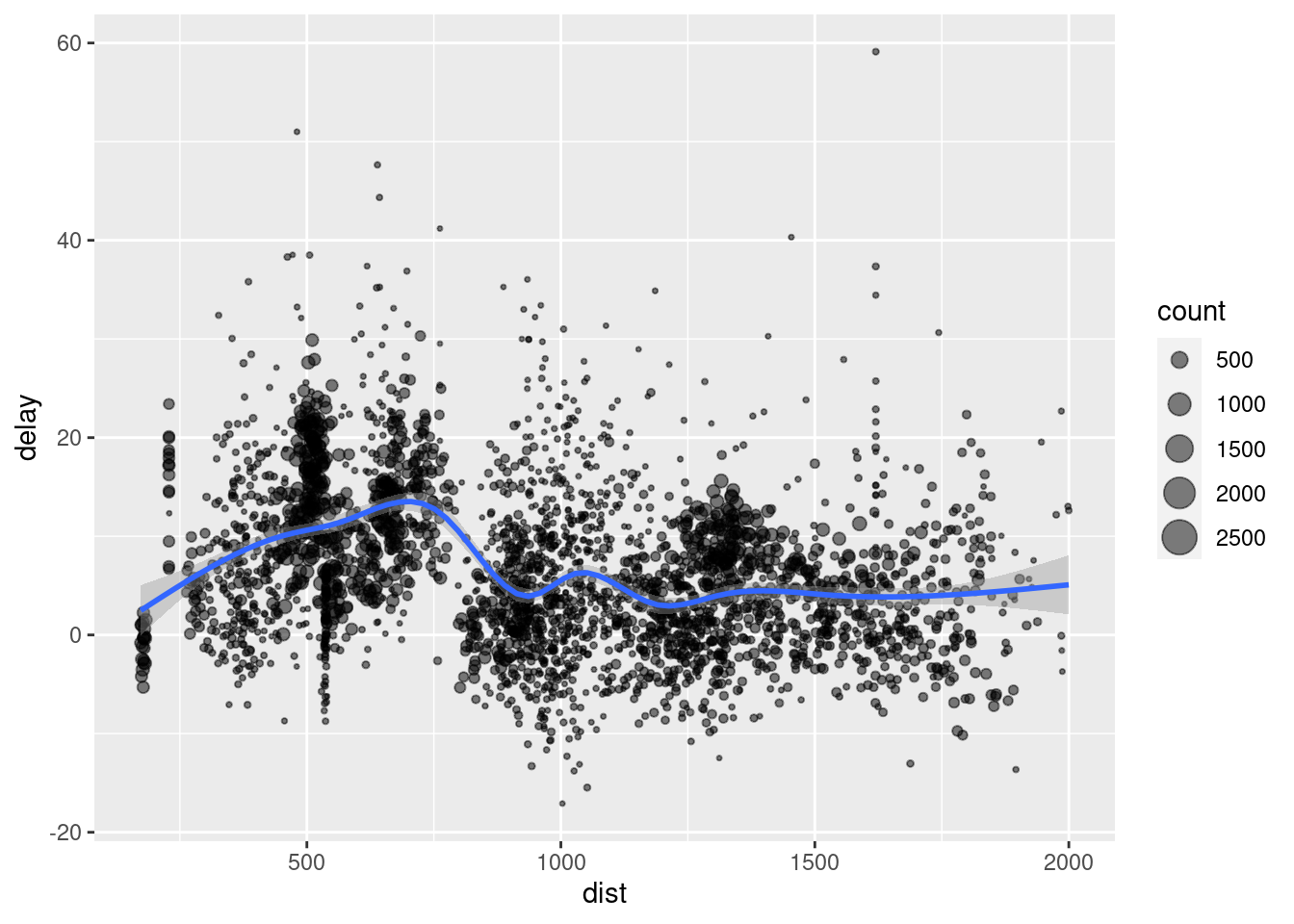
You use summarise() with aggregate functions, which take a vector of values and return a single number. There are many useful examples of such functions in base R like min(), max(), mean(), sum(), sd(), median(), and IQR(). dplyr provides a handful of others:
n(): the number of observations in the current groupn_distinct(x):the number of unique values in x.first(x),last(x)andnth(x, n)- these work similarly tox[1],x[length(x)], andx[n]but give you more control over the result if the value is missing.
Exercise 9. Find the number of planes and the number of flights that go to each possible destination (dest).
## # A tibble: 105 x 3
##    dest  planes flights
##    <chr>  <int>   <int>
##  1 ABQ      108     254
##  2 ACK       58     265
##  3 ALB      172     439
##  4 ANC        6       8
##  5 ATL     1180   17215
##  6 AUS      993    2439
##  7 AVL      159     275
##  8 BDL      186     443
##  9 BGR       46     375
## 10 BHM       45     297
## # … with 95 more rows
There is more information about dplyr on the website but it may be too advanced for what we need in the course.