2 First steps

R is an environment for statistical analysis, including gathering, modelling and visualizing data. We also call R the programming language used on this environment (http://www.r-project.org/).

2.1 Programming in R

Why you should use R?

Free and open
It includes lots of tools for plots
There is an interface, RStudio, which makes R projects very comfortable
Available on Windows, Mac and Linux
Console, scripts and notebooks available
Updated with state-of-art methodologies
Users community.

What trouble you will find.

It is really difficult become an expert on every aspects of R
Maintenance of codes will be hard if the language is used unproperly
Execution can be very slow if the language is used unproperly
Too much RAM can be needed

There are several tools that can be used for programming in R. The most spread one is RStudio. The company behind this software provides users with a very complete free version. They also work on several tools for R but independently from the R project.

Copy and pasting is a great way for developing good scripts. RStudio have written several cheatsheets with key content to getting started with some of the R tools. We may get some help from them. Go and visit their website.

2.2 R as a calculator

Our first approach to R will be using it as a calculator. Later on, we will begin taking advantage of it as a programming language. The main idea of these first lines is that we can compute both easy and complex calculations using the console of RStudio (some comments about RStudio IDE will be given during the lessons).

We can compute elementary mathematical operations, with common notation.

For more complex operations we need functions. Functions (in any programming language) are pieces of code that make some operations. We’ll get into them later on in the course. For now, it is enough knowing that R provide us with a lot of functions to make lots of calculations.

## [1] 120

## [1] 1.224647e-16

Suppose we want to calculate the force that is needed if we want to move an object of 9.5 $kg$ with an accelaration of 4.7 $m/{s^2}$. Newton’s second law may help: $F = m\cdot a$.

9.5 * 4.7

## [1] 44.65

Yeah! Cool, we did it! We now know that 44.65 $N$ are needed to move the object. The thing is that we will need to repeat the operation every time we desire to see the result. Avoiding that repetition can be achieved giving a name to that operation. newton seems a nice selection. We do this by using the <- symbol.

newton <- 9.5 * 4.7
newton

## [1] 44.65

Now, every time we write newton on the console we will get that result. In fact, on the upper right side of our RStudio windows we will see that something called newton has appeared, with a value of 44.65.

This idea can also be applied to the mass and the acceleration. We should define something with the mass value and another something with the acceleration value. In the future we will understand why this is so important.

acc <- 4.7
mass <- 9.5
newton <- mass * acc
newton

## [1] 44.65

Exercises.

Change the values of acc and mass (make sure on the upper right corner of RStudio that you have actually changed them). Write on the console newton. Try to understand what is necessary for successfully getting that changed.
What happens if you use = instead of <-? We will get into this by the end of the course. The idea right now is that the former is the one chosen as a good-practice standard.
You have defined acc. Type ACC and see what happens when you try to work with it.

2.3 Simple types of objects

When programming (not only with R but in general) we will use elements such as 3, -2.5, "cool_element", a_function_with_nice_properties()… They are different in many ways but they all are objects for R. R understands that both 3 and "cool_element" are things with different properties. For instance, you can add 3 and 2 but can’t 3 and "cool_element". These properties the thing (or object) has are what make it belong to a class or other. 3 in the real life is a number and "cool_element" is text. R needs to know that so that it will work differently with both of them. To do this, 3 belongs to the class numeric and "cool_element" to the class character (commonly called string in other languages). We’ll get into details in the next lines.

When we want to know what type of object we’re working with we’ll use the function class(). Let’s get into details.

Remark. When the documentation about a funcion is needed, is easily accesible via ? name_of_the_function, e.g., ? class. The focus of RStudio will move to the tab Help, on the lower left side of the window, by default.

2.3.1 Numeric

We have already seen some examples with numbers in R.

1
2.3
-1003.65
pi

2.3.1.1 Integer

Remember from high school the differences between real and integer numbers. 1, 1024, -53 are integers, but 0.5, -1.333 or $\pi$ aren’t. In R there exists a way of indicating such a difference and is important when dealing with large sets of data. The reason behind this is that R needs less information about an integer than about a real number. We will not get into the technical details in this course.

If we define a variable my_number as my_number <- 10, R will not understand the variable as integer, but a real number, therefore, numeric.

my_number <- 10
class(my_number)

## [1] "numeric"

For letting R know this variable should be define as integer, we use L.

my_number <- 10L
class(my_number)

## [1] "integer"

Numerical operations apply similarly to integer variables.

2.3.2 Character

Even though statistics deals always with numbers, saving text data is mandatory to understand what information we have. For example, we may have a table with population data of several cities, but we need to have those cities’ names to relate each piece of population data with the city. Thus, we need a way to tell R that a text is a text, so that it will understand it doesn’t have to work with it as if it were a number.

The way of doing this is "". Some examples:

city <- "Madrid"
capital_letters <- "NEW YORK"
a_number <- "10"
strange_characters <- "@!-/"
all_together <- "¿Cuál es la capital de España?"

class(city)

## [1] "character"

class(all_together)

## [1] "character"

We can also operate with character (or string) objects, generally with functions. We may see some examples in other sections but it is not a main goal of the course.

2.3.3 Logical

When programming, you will need to tell the computer to do something taking into account a condition. For example, creating a new folder if it doesn’t exists yet. Thus, R must know whether something is true or false. For this, we have the reserved words TRUE and FALSE (capital letters).

This is crucial when developing your own processes and functions but for now it’ll be enough getting the general idea.

saying_yes <- TRUE
class(saying_yes)

## [1] "logical"

Remark. Generally, the logical type is called boolean in other programming languages and it is easy finding documentation refering to this word, even about R.

Another remark. What the programming language hide behind a logical value is a number. TRUE equals 1 and FALSE equals 0.

We have seen some examples of operations with numbers but we can also compare them in the usual way.

pi > 3

## [1] TRUE

log10(100) == 2

## [1] TRUE

-3 <= -4

## [1] FALSE

TRUE == 1

## [1] TRUE

FALSE == 0

## [1] TRUE

TRUE == 3

## [1] FALSE

We can assign these comparisons to variables.

comparison1 <- pi > 3
comparison2 <- log10(100) == 2
comparison3 <- -3 <= -4

class(comparison1)

## [1] "logical"

class(comparison2)

## [1] "logical"

class(comparison3)

## [1] "logical"

We will see a practical example of this when introducing the tables (data frames).

2.4 Sets of elements

2.4.1 Vectors

In statistics we usually work with sets of data, i.e., several numbers. Imagine we have data about the height of several people and want to calculate the average height. We can pass this numbers to the R function mean(), which will return the desire result.

mean(1.75, 1.69, 1.81, 1.65, 2.01, 1.73, 1.90, 1.62)

## [1] 1.75

If we want to use that set again for another calculations (e.g., standard deviation with sd()), we need to define a new variable in R with those numbers. Writing them in the same way we have just done would return an error.

my_set <- 1.75, 1.69, 1.81, 1.65, 2.01, 1.73, 1.90, 1.62
# Error: unexpected ',' in "my_set <- 1.75,"

For managing R to understand those numbers should be saved in the same variable all together, with need the c() function.

my_set <- c(1.75, 1.69, 1.81, 1.65, 2.01, 1.73, 1.90, 1.62)
my_set

## [1] 1.75 1.69 1.81 1.65 2.01 1.73 1.90 1.62

mean(my_set)

## [1] 1.77

sd(my_set)

## [1] 0.1316923

The avarage height is 1.77 meters and the standard deviation is 13 centimeters.

These sets of elements are called vectors. A vector in R is a set of objects of the same type. However, if ask R about the class of a vector, it will say the class is the one of the elements.

class(c(2, 4, 6))

## [1] "numeric"

class(c("hi there!", "I don't really understand this R stuff", "abc10"))

## [1] "character"

class(c(TRUE, TRUE, FALSE, TRUE, FALSE))

## [1] "logical"

The length of the vector is the number of elements it contains and can be consuted with the length() function. We can extract individual elements from a vector or subsets of it with squared brackets ([]) and the desired indexes. The index of the first element of the vector is 1. For several programming languages, such as Python the first index is 0.

my_set[2]

## [1] 1.69

my_desired_index <- 3
my_set[my_desired_index]

## [1] 1.81

Be careful with the notation when mixing vector and functions.

my_set[length(my_set)]

## [1] 1.62

There is no element in the vector whose index is 0.

my_set[0]

## numeric(0)

For subsetting instead of extracting indivual elements, we need to provided the [] with another vector, whose numbers will be the indexes of the elements we want.

my_indexes <- c(2, 4, 6)
my_set[my_indexes]

## [1] 1.69 1.65 1.73

my_set[-my_indexes] ## all except my_indexes

## [1] 1.75 1.81 2.01 1.90 1.62

For simplyfing, there is no need on writing c(1, 2, 3, 4, 5). You can use the sequence notation 1:5.

a <- 1:5
b <- c(1, 2, 3, 4, 5)

a == b ## element by element

## [1] TRUE TRUE TRUE TRUE TRUE

## [1] 1 2 3 4 5

Exercise. What happens when you define a variable with the name c? Bear in mind that c() is a function in R. Spoiler alert. Not much: you just need to be careful and remember you have two different things with the same name, but there wil be no ambiguity since the uses of one of them are different form the other’s.

You can also use this : notation for indexes, as well as logical vectors and integers variables.

my_set[4L]

## [1] 1.65

logical_vector <- c(TRUE, FALSE, TRUE, FALSE, TRUE, FALSE, TRUE, FALSE)
my_set[logical_vector]

## [1] 1.75 1.81 2.01 1.90

Notice that, in the logical indexes case, the length of the index vector and the main vector are the same. This doesn’t have to be like this always, since R knows how to recycle information, though it may be counterintuitive is some ocasions.

my_set[c(TRUE, FALSE)]

## [1] 1.75 1.81 2.01 1.90

my_set[c(TRUE, FALSE, TRUE)]

## [1] 1.75 1.81 1.65 1.73 1.90

2.4.2 Matrix

You may have studied matrixes back in high school but for us we will understand them as tables with elements, distributed along rows and columns. As well as we saw with vectors, the elements of a matrix must belong all to the same class.

Vectors were defined via c() but there is no way of indicating a second dimension to this function, so that we can have rows and columns. For achieving this, we use matrix().

my_matrix <- matrix(c(10, 12, 9, 1, 5, 7, -1, -6, 8, 100, 200, 300), nrow = 3)
my_matrix

##      [,1] [,2] [,3] [,4]
## [1,]   10    1   -1  100
## [2,]   12    5   -6  200
## [3,]    9    7    8  300

There are several considerations that must be taken into account when defining matrixes but we won’t get into them in this course since we will focus on data frames. We’ll just mention a couple of thigs related with working already defined matrixes.

A vector has one only dimension and the number of elements is its length. For matrixes, there is no length concept. Instead, we work with rows and columns.

nrow(my_matrix)

## [1] 3

ncol(my_matrix)

## [1] 4

We have tow dimensions, therefore we need to specify two indexes when extracting elements.

desired_row <- 2
desired_column <- 4

my_matrix[2, 4]

## [1] 200

Of course, vectors can also be used as indexes for submatrixes.

my_matrix[1:2, 3:4]

##      [,1] [,2]
## [1,]   -1  100
## [2,]   -6  200

2.4.3 Data frames

In statistics, a popular format for keeping data are tables. In R, the main type of tables is called data frame. A data frame is a table, as well as matrixes, but its elements don’t have to be all of the same type. The first column can contain integers, the second, characters, the third, numbers, the fourth, logicals, and so on.

my_data_frame <- data.frame(
  col1 = 1:4, 
  col2 = c("Category 1", "Category 2", "Category 3", "Category 4"), 
  col3 = c(3.4, -2.5, 10.1, -0.05), 
  col4 = c(T, F, F, T)
)

my_data_frame

##   col1       col2  col3  col4
## 1    1 Category 1  3.40  TRUE
## 2    2 Category 2 -2.50 FALSE
## 3    3 Category 3 10.10 FALSE
## 4    4 Category 4 -0.05  TRUE

Exercises.

Check the type of each column for the data frame you’ve just created. Remember you need the function class() to do it.
Is there anything strange with the second column? What were you expecting? Ask your teach about this and feel free to read ? factor but don’t worry about it for now. We’ll get into that later.

Data frames have some things in common with matrixes. They are both tables, therefore the same sintax can be used to get their elements:

my_data_frame[1, 2] # first row, second column

## [1] "Category 1"

my_data_frame[2:4, 2] # second to fourth rows, second column

## [1] "Category 2" "Category 3" "Category 4"

my_data_frame[1:3, -4] # first to third rows (included), all except fourth column

##   col1       col2 col3
## 1    1 Category 1  3.4
## 2    2 Category 2 -2.5
## 3    3 Category 3 10.1

Exercise. What are the types of objects returned with those executions.

As you may have realized, this is a bit messy for beginning working with R. We have mentioned it because it is important to know that this exist, but we will not work with data frames as matrix, but we’ll use the proper tools for data frames that R provides.

First of all, we need to understand how to extract one column in the form of a vector.

2.4.3.1 `$` and `[[`

You may have noticed that we defined our dataframe with named columns: col1, col2 and so on (it is worth mentioning that this names can be whatever you desire, following some rules we’ll not describe now). This is very convenient since it makes easy getting the elements from each column:

my_data_frame$col1

## [1] 1 2 3 4

my_data_frame[["col1"]]

## [1] 1 2 3 4

$ has the advantage of autocompletion (with Tab).
[[ has the advantage of parametrizing via characters, something very useful when dealing with functions, mainly by the end of the course.

There are several ways of verifying those vector are equal. We choose this one:

dollar_sintax <- my_data_frame$col1
double_bracket_sintax <- my_data_frame[["col1"]]

all(dollar_sintax == double_bracket_sintax)

## [1] TRUE

we could have done it at a glance but if you have a one million column data frame, this way’s better ;)

Remark. Notice we typed double squared bracket ([[), not single ([). The character notation can also be used in the second case but differently and there are more cases to be considered. For simplicity’s sake, we won’t get into that.

We don’t know yet how to read data from files (patience, my dear reader) but R makes comfortable using some preloaded datasets as examples. A classical one is iris, a dataset with a some of flowers of three species and some info about them. We will use as a example for a while.

First we should have an idea about the general structure of the data frame. We can type iris on the console and see the data but it is not very clarifying, since there are too many data and don’t fit tidily inside the tab.

A common function for a first approach is head().

head(iris)

##   Sepal.Length Sepal.Width Petal.Length Petal.Width Species
## 1          5.1         3.5          1.4         0.2  setosa
## 2          4.9         3.0          1.4         0.2  setosa
## 3          4.7         3.2          1.3         0.2  setosa
## 4          4.6         3.1          1.5         0.2  setosa
## 5          5.0         3.6          1.4         0.2  setosa
## 6          5.4         3.9          1.7         0.4  setosa

Cool. head() shows by default the first six rows of the data frame used as input (be careful if you have too many columns). The analogous is tail(), which shows the last six rows. This number is a parameter of the function and can be redefined.

tail(iris, 10)

##     Sepal.Length Sepal.Width Petal.Length Petal.Width   Species
## 141          6.7         3.1          5.6         2.4 virginica
## 142          6.9         3.1          5.1         2.3 virginica
## 143          5.8         2.7          5.1         1.9 virginica
## 144          6.8         3.2          5.9         2.3 virginica
## 145          6.7         3.3          5.7         2.5 virginica
## 146          6.7         3.0          5.2         2.3 virginica
## 147          6.3         2.5          5.0         1.9 virginica
## 148          6.5         3.0          5.2         2.0 virginica
## 149          6.2         3.4          5.4         2.3 virginica
## 150          5.9         3.0          5.1         1.8 virginica

For checking the number of rows and columns of the data frame (these ones also work with matrixes):

nrow(iris)

## [1] 150

ncol(iris)

## [1] 5

dim(iris)

## [1] 150   5

We have easily verified there are 150 rows and 5 columns. If we want to know what columns there are, we can get their names with names():

names(iris)

## [1] "Sepal.Length" "Sepal.Width"  "Petal.Length" "Petal.Width"  "Species"

We have info about the sepal, the petal and the species each flower belongs to. We could have also used colnames() for this. Bear in mind that this one would also work with matrixes but the former wouldn’t.

We’ll come back later to have a look at the structure of a data frame with new tools. For now, let’s go on with the $ notation.

iris is a data frame.

class(iris)

## [1] "data.frame"

But its columns, from an independent point of view, are vectors. Therefore, their classes are the ones of their elements.

class(iris$Sepal.Length)

## [1] "numeric"

class(iris$Sepal.Width)

## [1] "numeric"

class(iris$Petal.Length)

## [1] "numeric"

class(iris$Petal.Width)

## [1] "numeric"

class(iris$Species)

## [1] "factor"

We have some numbers and characters (again, don’t worry about the factor thing yet. We’ll come to that). A typical function to get a general idea of the distributions of the columns is summary().

summary(iris)

##   Sepal.Length    Sepal.Width     Petal.Length    Petal.Width   
##  Min.   :4.300   Min.   :2.000   Min.   :1.000   Min.   :0.100  
##  1st Qu.:5.100   1st Qu.:2.800   1st Qu.:1.600   1st Qu.:0.300  
##  Median :5.800   Median :3.000   Median :4.350   Median :1.300  
##  Mean   :5.843   Mean   :3.057   Mean   :3.758   Mean   :1.199  
##  3rd Qu.:6.400   3rd Qu.:3.300   3rd Qu.:5.100   3rd Qu.:1.800  
##  Max.   :7.900   Max.   :4.400   Max.   :6.900   Max.   :2.500  
##        Species  
##  setosa    :50  
##  versicolor:50  
##  virginica :50  
##                 
##                 
##

Let’s count the number of flowers with a longer sepal than the mean (5.8, according to the summary).

First we need to know, for each row, whether the sepal length is greater than 5.8: iris$Sepal.Length > 5.8.
That piece of code will return a vector of 150 TRUE or FALSE values, indicating what we want to know.
Now we need to count how many trues there are. But remember that TRUE == 1, so a good way to counting is adding all the TRUE cases, with sum().

sum(iris$Sepal.Length > 5.8)

## [1] 70

There is no need in typing the mean manually. You can use the function mean() instead.

my_average <- mean(iris$Sepal.Length)
sum(iris$Sepal.Length > my_average)

## [1] 70

This is an example of comparing every row with the same number. But you can use different values for each row. For example, let’s count the number of flowers whose sepal is longer than its petal.

sum(iris$Sepal.Length > iris$Petal.Length)

## [1] 150

All of them. Naïve example.

We can also use these logical vectors to extract subvectors with information. For instance, let’s print the sepal length of the flowers whose petal width is above the median:

my_index <- iris$Petal.Width > median(iris$Petal.Width) # is above the median

head(my_index) # these are logical values indicating whether the flower corresponds with the filter

## [1] FALSE FALSE FALSE FALSE FALSE FALSE

iris$Sepal.Length[my_index]

##  [1] 7.0 6.4 6.9 6.5 6.3 5.2 5.9 6.1 6.7 5.6 6.2 5.9 6.3 6.6 6.8 6.7 6.0 6.0 5.4
## [20] 6.0 6.7 6.1 6.3 5.8 7.1 6.3 6.5 7.6 4.9 7.3 6.7 7.2 6.5 6.4 6.8 5.7 5.8 6.4
## [39] 6.5 7.7 7.7 6.0 6.9 5.6 7.7 6.3 6.7 7.2 6.2 6.1 6.4 7.2 7.4 7.9 6.4 6.3 6.1
## [58] 7.7 6.3 6.4 6.0 6.9 6.7 6.9 5.8 6.8 6.7 6.7 6.3 6.5 6.2 5.9

Now we have a subvector of the sepal length. Let’s count the number of flowers with this caracteristic. This will be the number of elements in the vector, what we can calculate with length().

length(iris$Sepal.Length[my_index] )

## [1] 72

There are 72 flowers whose petal width is above the median.

Exercises.

Count the number of flowers with Petal.Length higher than 5.1

sum(iris$Petal.Length > 5.1)

## [1] 34

Check which species have flowers with sepal width higher than 3.5 and lower than 4. Hint. & will be needed when more than one condition is needed. Besides, for simplifying the result you may need unique(). Use ? for details.

unique(iris$Species[iris$Sepal.Width > 3.5 & iris$Sepal.Width < 4])

## [1] setosa    virginica
## Levels: setosa versicolor virginica

How many flowers of each species are there? Hint. Function table() may be useful.

table(iris$Species)

## 
##     setosa versicolor  virginica 
##         50         50         50

Calculate the sepal width average of the flowers whose sepal width is below average.

mean(iris$Sepal.Length[iris$Sepal.Width < mean(iris$Sepal.Width)])

## [1] 5.972289

Calculate the median of the petal width for each species separetely.

print("Setosa:")

## [1] "Setosa:"

median(iris$Petal.Width[iris$Species == "setosa"])

## [1] 0.2

print("Versicolor:")

## [1] "Versicolor:"

median(iris$Petal.Width[iris$Species == "versicolor"])

## [1] 1.3

print("Virginica:")

## [1] "Virginica:"

median(iris$Petal.Width[iris$Species == "virginica"])

## [1] 2

Calculate the minimum and maximum petal length for every versicolor flower. Then count how many setosa and virginica flowers there are with the petal length between those values.

print("Min:")

## [1] "Min:"

minimo_valor <- min(iris$Petal.Length[iris$Species == "versicolor"])
minimo_valor

## [1] 3

print("Max:")

## [1] "Max:"

maximo_valor <- max(iris$Petal.Length[iris$Species == "versicolor"])
maximo_valor

## [1] 5.1

print("Versicolor:")

## [1] "Versicolor:"

especie <- "setosa"
logical_for_especie <- iris$Species == especie
petal_lengths_for_especie <- iris$Petal.Length[logical_for_especie]

true_si_mayor_que_min <- petal_lengths_for_especie > minimo_valor
true_si_menor_que_max <- petal_lengths_for_especie < maximo_valor

# Casos que cumplen ambas cosas:
# Esto es un vector lógico: true_si_mayor_que_min & true_si_menor_que_max
# Puedo sumar los valores para hacer el conteo:
sum(true_si_mayor_que_min & true_si_menor_que_max)

## [1] 0

print("Virginica:")

## [1] "Virginica:"

especie <- "virginica"
logical_for_especie <- iris$Species == especie
petal_lengths_for_especie <- iris$Petal.Length[logical_for_especie]

true_si_mayor_que_min <- petal_lengths_for_especie > minimo_valor
true_si_menor_que_max <- petal_lengths_for_especie < maximo_valor

sum(true_si_mayor_que_min & true_si_menor_que_max)

## [1] 9

What happens if you use plot() with the data frame iris?

plot(iris)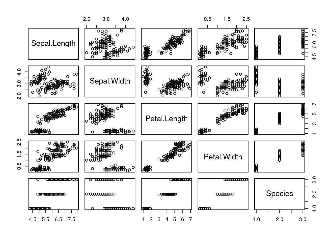

If you type Titanic on the console you will set a data set with a not too comfortable format for analysis. Use as.data.frame() to convert it to a data frame and assign it to a new variable (object) in R (pick a name of your choice). Now that data frame is on memory.

df_titanic <- as.data.frame(Titanic)

Verify that data frame is in fact a data frame.

class(df_titanic)

## [1] "data.frame"

Check the classes of the data frame’s columns

class(df_titanic$Class)

## [1] "factor"

class(df_titanic$Sex)

## [1] "factor"

class(df_titanic$Age)

## [1] "factor"

class(df_titanic$Survived)

## [1] "factor"

class(df_titanic$Freq)

## [1] "numeric"

Count (or sum) the number of people who survived and the number of people who didn’t. If you have questions about the data, type ? Titanic to get into the help (yes! You also have help for datasets.).

print("Survived:")

## [1] "Survived:"

sum(df_titanic$Freq[df_titanic$Survived == "Yes"])

## [1] 711

print("Didn't survive")

## [1] "Didn't survive"

sum(df_titanic$Freq[df_titanic$Survived == "No"])

## [1] 1490

Count the number of children who were on the ship.

sum(df_titanic$Freq[df_titanic$Age == "Child"])

## [1] 109

Count the number of men from first class.

## [1] 180

Were there any children among the crew? And women?

print("Children:")

## [1] "Children:"

sum(df_titanic$Freq[df_titanic$Age == "Child" & df_titanic$Class == "Crew"])

## [1] 0

print("Women:")

## [1] "Women:"

sum(df_titanic$Freq[df_titanic$Sex == "Female" & df_titanic$Class == "Crew"])

## [1] 23

2.5 Extending R with libraries

What we’ve seen so far belongs to what it is known as R base. When programming in R, we’ll use a set of words and symbols that the computer understands and operates according to them. But because of the complexity of the projects that are usually developed in Data Science, programming everything in R base may become verbose, difficult and the least practical way of working.

Several people from the R community work continously developing sets of code that, with new words and symbols, expand R and its uses. These sets of code are called libraries or packages (not only in R but in every programming language, such as Python).

For using a library, we employ the function library(), with the name of the desired library as the parameter.

For instance, we have seen the data.frame structure. If we want to build a data frame from scratch we will type data.frame(), with some data between the brackets. However, there are other types of data frames in R, which are more efficient from a couple of point of views (we will explain these during the sessions, probably). In this course, we are going to use one of these types: the tibble.

Tibbles are redefined data frames and the way of building one is similar: we type tibble(), with the data in form of vectors inside the brackets. The problem is that if we type that directly, we’ll get an error:

tibble(
  my_cool_column = c(23, 56, 77), 
  my_lovely_column = c("thing1", "thing2", "thing3")
)

# Error...: could not find function "tibble"

R is telling us that there is no such a function tibble(). In fact, there isn’t… at least in R base. There is one tibble() function in some other place: in one library (or several, but we’ll get into that later on).

library(tibble)

tibble(
  my_cool_column = c(23, 56, 77), 
  my_lovely_column = c("thing1", "thing2", "thing3")
)

## # A tibble: 3 x 2
##   my_cool_column my_lovely_column
##            <dbl> <chr>           
## 1             23 thing1          
## 2             56 thing2          
## 3             77 thing3

Now it works. We’ll study tibbles during the sessions. The important thing to be remembered R base will not be a comfortable tool for our data science projects alone: we will need it expanded. And the way for achieving this are libraries.

2.6 Installation

Remark. The code above may not have worked in your local computer. You need to install a library before using it.

Installing libraries (or packages: two words, same thing) is required in order to make use of them. In general, all we need to do is typing install.package(). Between the brackets we will include the name of library with quotation marks.

install.packages("tibble")

Recommendation. Once you install a library on your computer, there is no need to do it again. It is strongly recommended to type the installation command on the console, not on your scripts, so that the library won’t be reinstalled all over again.

Exercise. During the session, if you pay attention, we will talk about the tidyverse. It is a set of libraries, containing the two most important for our course: dplyr and ggplot2. Installing tidyverse, dplyr, ggplot2, tibble, readr and a lot more will also be intalled along. Install tidyverse on your computer. Remember to use the console. Hint. When you install a library, a lot of messages will come up on the console. Don’t worry: they are only messages, not errors. If you really read the word Error on the console, ask your teacher.

2 First steps

2.1 Programming in R

2.2 R as a calculator

2.3 Simple types of objects

2.3.1 Numeric

2.3.1.1 Integer

2.3.2 Character

2.3.3 Logical

2.4 Sets of elements

2.4.1 Vectors

2.4.2 Matrix

2.4.3 Data frames

2.4.3.1 $ and [[

2.5 Extending R with libraries

2.6 Installation

2.4.3.1 `$` and `[[`